6.2. How to use HORTON’s matrix package?

6.2.1. Introduction

In HORTON, we use our own matrix package (abstraction layer) to implement the linear algebra code (low-level code) into the quantum chemistry code (high-level code). There are two main reasons for such an architecture:

1. We can develop new linear algebra operations without breaking the higher-level code. For example, if we implemented Cholesky decomposition for the transformation of 2-electron integrals, we should be able to use this method in the geminals code without rewriting this code.
2. Numpy, the conventional linear algebra package in Python, may not manage memory effectively for large objects, such as the 2-electron integrals. For example, Numpy allocates temporary memory when evaluating a += b, which is costly when a or b is very large. By developing a matrix package (using the Numpy package), we gear towards memory management of quantum chemistry calculations. So, the matrix package is used instead of Numpy package directly.

Although such an abstraction layer seems pedantic and ostentatious, requiring a tedious implementation of all new operations into the matrix package, the small penalty in performance and the ease of implementing different concepts into the low-level areas of HORTON make it well worth the effort.

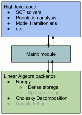
The image below represents this architecture schematically (the gray bullet points are future implementations).

6.2.2. Using the matrix package

The package horton.matrix is organized as follows:

The package consists of backend modules, each with their own implementation of the data storage and data manipulation. So far, there are two such modules: a dense Numpy storage and Cholesky decomposition of the Numpy storage. Because these modules treat data fundamentally differently, the corresponding methods for manipulating the data, as listed in base.py, should be implemented separately. These methods are used by the high-level modules.

The code for each module is structured by the type of data that is manipulated within a class. So far, classes for 1-index tensor, 2-index tensor, 3-index tensor, 4-index tensor, and wavefunction expansion have been implemented.

To avoid reallocation of memory, we use a LinalgFactory instance to create these objects (e.g. 2-index tensor). This instance will allocate memory for these objects, and then, the operations performed on these objects will modify their own attributes directly. Most of the operations are in-place, i.e. modifying their own data based on input and not returning any output.

For example, to create and modify a dense 2-index tensor, we first create a DenseLinalgFactory instance and call it lf:

lf = DenseLinalgFactory()

Then, we use lf to allocate a 2-index tensor object:

A = lf.create_two_index()      # 2-index tensor

Now, we can modify the 2-index tensor object by some in-place operations:

A.iadd(B)         # A = A + B
A.idot(B)         # A = A * B

# A = B + C is not a possible in-place operation, but doable in two steps:
A.iadd(B)         # A = A + B
A.iadd(C)         # A = A + C

Note that more complex operations, such as A = B + C, can be broken up into a series of in-place operations, that deal with the explicitly allocated memory.

We can also allocate other implemented objects using lf:

A4 = lf.create_four_index()    # 4-index tensor
wfn = lf.create_expansion()    # wavefunction expansion

Furthermore, we can pass lf as an argument to other parts of the code, where it is used to allocate an object, like,

er = obasis.compute_electron_repulsion(lf)

We can appreciate the simplicity of implementing different modules by playing with the different backend modules available. For example, instead of the DenseLinalgFactory, we could have used,

lf = CholeskyLinalgFactory()

Making this change will not change any of the preceding code, provided that the same methods and attributes are implemented in this module as well.

Many functions and classes have been implemented into the matrix package. It may help to read over some of the documented module files in horton.matrix.dense and horton.matrix.cholesky to see if a desired function has already been implemented.